


1. INTRODUCTION
According to the recent trend of reducing weight and improving fuel efficiency, it is required to extend the limits of extreme engine downsizing in the automotive industry [1,2]. At the same time, despite the engine downsizing, high output engines are also in demand. For those reasons, the fasteners that connect elements of the engines have to be durable and lightweight. In particular, the connecting rod fastener bolts and cylinder head bolts must withstand tougher conditions in terms of high temperatures and pressures during engine operation [3]. Hence, worldwide steelmakers have focused on developing ultra-high strength fasteners (class 14.8, 15.8 and 16.8). Some domestic enterprises have also been studying the development and mass-production of class 16.8 steels using a cold forging process. Cold forging has various advantages compared to the hot forming process, including the geometrical precision of components, excellent surface finish, high production rate, etc. [4,5,6].
This study is a part of the research aimed at manufacturing bolts which have a 1,600 MPa tensile strength using a cold heading process. For high strength bolts, medium carbon steels are widely used with some added alloy elements, such as Cr, Mo, and Mn [7]. After the hot-rolling and cooling process, the microstructure of the wire rods consists of ferrite and pearlite. The lamella structure of pearlite is not ductile enough for cold forging [8]. Therefore, spheroidization annealing is conducted to convert the cementite in pearlite into a spherical shape, which improves cold formability and the machinability of the material prior to the forming process. For the spheroidization annealing of steel wires, the Subcritical and the Intercritical annealing processes are mainly used in practice [9].
The mechanisms and annealing process of spheroidization annealing have been researched for decades. As the importance of the steel manufacturing process increases, many studies on the details and conditions of spheroidization annealing are being actively conducted. For example, the effect of spheroidization annealing can differ depending on the annealing temperature, heating time, and many other process parameters, and it is not well known what the best options for the spheroidization annealing effect is.
To manufacture ultra-high strength bolts of 16.8 class or higher, not only an alloy design for ultra-high strength but also a spheroidization heat treatment process is essential to make the wire into a bolt shape. However, in the current industry, spheroidization heat treatment is carried out using conventional heat treatment methods without fully considering the composition and characteristics of each material. By finding an optimized spheroidization heat treatment method for each material, industry can save unnecessary process costs and time to reach the target strength after heat treatment.
In order to find the optimized spheroidization heat treatment, it is necessary to set the control parameters of the spheroidization heat treatment process. Then, it is necessary to know how and to what extent those control parameters affect the strength of the material. Thus, in this work, we investigated the parameters and their effects on the optimization of the annealing process. We also present a new quantitative measurement method to evaluate the degree of spheroidization using data analysis.
2. EXPERIMENTAL
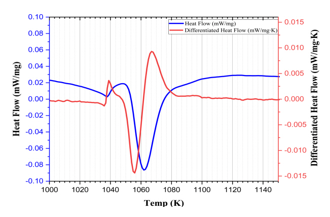
The material used in this study was hot-rolled medium carbon Cr-Mo steel wire rods (8 mm in diameter), and the chemical compositions of the steel are given in Table 1. To design a suitable spheroidization heat treatment condition for the steel, it is necessary to accurately measure the Ac1 and Ac3 temperature of the steel. The Ac1 temperature is the temperature at which the austenite phase starts to transform from the ferrite phase (α+pearlite→α+γ). And, the Ac3 temperature is the temperature at which the austenite is completely transformed from the ferrite phase (α+γ→γ). The Ac1 and Ac3 temperatures of the steel were measured using a differential scanning calorimeter (DSC, DSC 404 F1, Pegasus) under an Ar atmosphere. The DSC basically measures heat changes in the sample. A sample undergoes thermal changes as its phase changes, so it is possible to check its phase transformation as the temperature increases or decreases using DSC [10-12]. Since the transformation temperature is a function of heating rate, in this research, they were measured during heating at a rate of 5 K/min [13,14].
Fig 1 is a specific interval of the DSC curve used to determine the transformation temperature of the steel. The two temperature points appear due to an abrupt change in the gradient of the heat flow, or the start and end points of the endo peak in the DSC curve [15]. In order to show this gradient change, a differentiated heat flow is presented as shown in Fig 1. The temperatures of Ac1 and Ac3 are 1053 K and 1083 K, respectively.
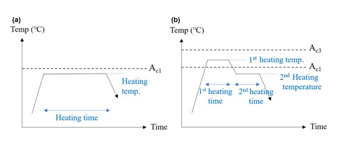
In order to compare various heat treatment conditions, the use of Subcritical annealing and Intercritical annealing, which are generally well-known spheroidization heat treatment methods, has been proposed. Subcritical annealing is a method of heat treatment for a certain period of time below the Ac1 temperature, and Intercritical annealing is a method of first heating between Ac1 and Ac3 temperatures and then applying a second heating below the Ac1 temperature.
Fig 2 schematically shows the two spheroidization heat treatment conditions used in the experiment. Fig 2 (a) is a schematic diagram of Subcritical annealing. As a method of heat treatment at an Ac1 temperature or lower, heat treatment conditions were designed by setting heating temperature and heating time as variables. Heating temperature refers to the temperature that is constantly maintained and the highest in the process, and heating time is the holding time at that temperature that is constantly maintained and the highest in the process, and heating time is the holding time at that temperature. Fig 2(b) is a schematic diagram of Intercritical annealing. In this method, a 1st heat treatment between Ac1 temperature and Ac3 is applied initially, with a 2nd heat treatment at Ac1 or lower.
The heat treatment was divided into two steps, and the heating temperature and heating time were set as variables for each heat treatment step to design heat treatment conditions. The highest holding temperature in the 1st heat treatment step is the 1st heating temperature, and the holding time is the 1st heating time, and the same applies to the second heat treatment step.
The heating rate of all the wires was 5 K/min. In the subcritical annealing, the wires were heated to 1003-1043 K, and held at this temperature for 3-20 hours. In the Intercritical annealing, the wires were first heated to 1063-1073 K and the holding time was 3-7 hours. Then, the wires were cooled to 1003-1043 K at a cooling rate of 3 K/min and maintained at this temperature for 3 hours. All the wires reached room temperature by furnace cooling after heat treatment. Table 2 shows the spheroidization heat treatment conditions applied to the wires in the experiment. In order to simulate the actual spheroidization heat treatment condition, the experiment was conducted in a commercial box-type furnace without any atmosphere control.
To analyze the various spheroidization heat treatment conditions, it is necessary to designate control parameters for each condition and classify them into various levels. In subcritical annealing, the heating temperature and time were selected for the two control parameters. The heating temperature was set to 3 levels, 1003, 1023, and 1043 K, and the heating time was set to 5 levels, 3, 5, 7, 10, and 20 hours. In the Intercritical annealing, four control parameters were selected: the 1st heating temperature and heating time, and the 2nd heating temperature and heating time. The 1st heating temperature was set to 2 levels, 1063 and 1073 K, and the 1st heating time was set to 3 levels, 3, 5, 7 hours. The 2nd heating temperature was set to 3 levels at 1003, 1023, and 1043 K, and the 2nd heating time was set to 1 level at 3 hours. Table 3 shows the control parameters and levels for each condition.
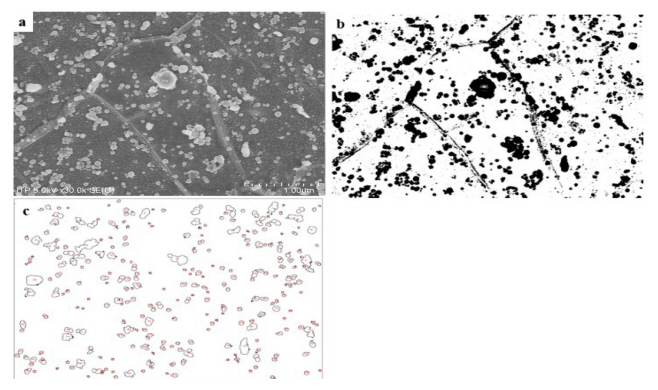
The SEM used for microstructure analysis was a HITACHISU-8010 with a resolution of 2.0-1.0 nm and a cold cathode field emission type electron gun. In this research, the microstructures of the steel were captured at an acceleration voltage of 5.0 kV at a 30,000X magnification. The microstructure used the ImageJ program for image analysis. The ImageJ is an open architecture program based on Java and can utilize various image analysis techniques [16, 17, 18]. Fig 3 shows the image analysis process of ImageJ based on the SEM image. In the SEM image Fig 3-(a), the spheroidized cementite has a brighter contrast than the base. In the ImageJ, only a specific contrast can be extracted by setting threshold. Through the extracted image, it is possible to analyze the aspect ratio, spheroidization rate, and spheroidization fraction of each spheroidized particle.
The Pearson correlation coefficient is a quantitative expression of the linear correlation between two variables [19]. In this research, the Pearson correlation coefficient was used to analyze the correlation between the spheroidized volume fraction of the steel and the surface hardness value. Nine of the Intercritical annealing conditions of the steel were randomly selected to calculate the spheroidized volume fraction using the SEM images, and a total of 90 data were used. The Pearson correlation coefficient analysis was performed using the corrgram and the Performance Analytics packages in the R program [20-22].
To analyze the optimal conditions for the spheroidization heat treatment of the steel, the surface hardness of each heat treatment condition was measured, and the S/N ratio (Signal to noise ratio) method and ANOVA were applied to the hardness data. In this research, hardness was measured to evaluate the characteristics of the spheroidized heat-treated steel for each condition. A total of 12 surface hardness values were measured around a concentric circle starting at half the length of the radius at the center of each sample, and then 10 surface hardness values were used, excluding the minimum and maximum values. The hardness of the specimen was compared using a micro Vickers hardness tester. SHIMADZU's HMV-G21ST can be used to measure the micro Vickers hardness of the specimen. The load of the indenter for measurement was set to HV0.3 (2.924N) and the holding time was set to 10 seconds.
Each result is converted into an S/N ratio. The steels require proper ductility and hardness degradation for post-cold heading, which is provided by spheroidization heat treatment. The spheroidization heat treatment results in a significant decrease in steel hardness. When converting this hardness value to an S/N ratio, ‘the smaller the better’ characteristics of the S/N ratio are required. Therefore, the S/N ratio is
where y is the performance characteristic value (surface hardness) and n is the number of y values.
ANOVA is an effective data analysis method that can be used to identify and determine the optimal process conditions, and the important control parameters needed to obtain the optimal quality of steels. For the experimental errors in the previous S/N ratio, the significance and independence test of the control parameters were calculated using the ANOVA. The experimental errors can be considered an effect due to the interaction of control parameters [23]. The control parameters can be considered significant parameters that affect the result value, if the effect on the result is sufficiently large compared to the experimental errors. Therefore, ANOVA uses experimental errors to identify the significant parameters that affect the results, and evaluates the confidence level of each control parameter. The ANOVA analysis was performed using the corrgram and Performance Analytics package in the R program [20-22].
3. RESULTS AND DISCUSSION
3.1 Hardness of the steel according to spheroidization heat treatment conditions
The surface hardness value of the Subcritical annealing is shown in Table 4. Fig 4 is a plot of the results of Table 4. The surface hardness values of the Subcritical annealing were widely distributed, from 140 HV (SA_15) to 277 HV (SA_1). The standard deviation value varied from 1.80 (SA_3) to 5.73 (SA_4). For steel that had not been previously heat treated, the surface hardness value was 412 HV. After heat treatment under all 15 conditions, a hardness degradation occurred, from 66% (SA_15) to 33% (SA_1).
In Fig 4, each graph represents the heating temperature, the x-axis represents the heating time and the y-axis represents the surface hardness value. When the heating temperature was the same, the longer the heating time, the greater the decrease in surface hardness. In addition, when the heating time was the same, the higher the heating temperature, the greater the decrease in surface hardness. This means that when the steel is carried out by Subcritical annealing, the total amount of heat applied must be increased to significantly degrade surface hardness. In particular, for heat treatment conditions at 1043 K, when the heating time was within 10 hours, the decrease in surface hardness degradation was not significant compared to other heat treatment conditions. However, after 20 hours, the surface hardness value was 140 HV, a significant decrease in surface hardness compared to heat treatment conditions with the same heating time.
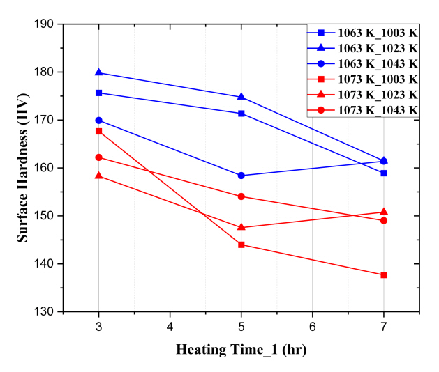
The surface hardness values for the Intercritical annealing are shown in Table 5. Fig 5 is a plot of the results of Table 5. The surface hardness values of the Intercritical annealing are distributed from 138 HV (IA_16) to 180 HV (IA_2). The standard deviation value is widely distributed, from 2.27 (IA_4) to 11.17 (IA_13). For steel which had not been previously heat treated, the surface hardness value was 412 HV. After heat treatment under all 18 conditions, the surface hardness value decreased from 65% (IA_16) to 56% (IA_2).
In Fig 5, each graph represents the heating temperature (1st heating temp_2nd heating temp), the x-axis represents the 1st heating time and the y-axis represents the surface hardness value. According to Fig 5, the hardness values of the conditions where the 1st heating temperature was 1073 K are lower than the conditions where the 1st heating temperature was 1063 K. So, as the 1st heating temperature increased, there was a significant degradation in surface hardness due to the spheroidization heat treatment. In addition, as the 1st heating time increased, the surface hardness generally decreased. Exceptionally, in the case of IA_9 and IA_17, the surface hardness increased about 3 HV compared to the heat treatment for 5 hours. However, these values fall within the standard deviation of each condition. Accordingly, for Intercritical annealing, as with Subcritical annealing, the surface hardness degraded more as the heating time increased.
When the 1st heating time was the same except for the 1st heating temperature, the surface hardness did not follow the same tendency as the Subcritical annealing. For (1073 K_1003 K), when the 1st heating time was 3 hours, the surface hardness was higher than the red plot of the same (1073 K_2nd heating time). But when the 1st heating time was 5 hours or more, the surface hardness was the lowest among all conditions. Therefore, unlike Subcritical annealing, for Intercritical annealing, the four control parameters had a complex effect on the steel due to the spheroidization heat treatment.
By comparing Fig 4 and Fig 5, it is possible to determine which spheroidization heat treatment conditions are suitable for the steel. Comparing only the surface hardness values, SA_15 had 140 HV and a standard deviation of 4.15, which was the lowest surface hardness for Subcritical annealing, but the heating time should be performed for 20 hours to reach the surface hardness value.
On the other hand, the surface hardness value of IA_16 has 138 HV and a standard deviation of 6.69, which was similar to SA_15, but the total heating time was 10 hours, which is much more efficient than Subcritical annealing. In addition, except for the conditions when heat treating for 20 hours in the Subcritical annealing, the surface hardness values under the Subcritical annealing were in the range of 197-277 HV, while the surface hardness values under Intercritical annealing were in the range of 138-180 HV. Therefore, for steel, Intercritical annealing is more efficient in terms of time cost and the surface hardness degradation.
3.2 Analysis of the relationship between the surface hardness and the spheroidized volume fraction
The surface hardness under various Subcritical annealing and Intercritical annealing conditions was measured, and as a result, the surface hardness value of the Intercritical annealing was determined to be significantly lower than the surface hardness value of the Subcritical annealing compared to the heating time. With general spheroidization heat treatment, the larger the degree of spheroidization, the greater the decrease in surface hardness.
In order to analyze the difference in surface hardness according to the degree of spheroidization, the microstructure of the specimen under the Intercritical annealing condition, where the surface hardness was greatly degraded, was photographed with a Scanning Electron Microscope (SEM). 9 of the 18 conditions, IA_1, IA_5, IA_3, IA_10, IA_9, IA_7, IA_15, and IA_14 were randomly selected and 10 SEM images per condition were obtained from arbitrary regions. Fig 6 shows 8 SEM images out of 90 SEM images obtained under each condition. The upper left of Fig 6 shows the heat treatment conditions and the surface hardness values of the corresponding image. Comparing IA_1 and IA_14, the larger the surface hardness value, the less spheroidized particles are observed. And the smaller the surface hardness value, the more spheroidized particles are observed. Therefore, the spheroidization heat treatment affects the surface hardness value, and the more spheroidized particles, the greater the surface hardness degradation, qualitatively.
In order to quantitatively analyze the relationship between the degree of spheroidization and the surface hardness, the degree of spheroidization was first quantitatively expressed. The expression of the degree of spheroidized particles can be mainly divided into spheroidal ratio and spheroidized volume fraction. The spheroidal ratio means how close the spheroidized particles are to a circle, that is, the aspect ratio of the particles. The closer the aspect ratio is to 1, the closer the spheroidal ratio is to 1. The spheroidized volume fraction refers to the ratio of spheroidized particles to the matrix in a specific area. According to Fig 6, since the aspect ratio of the spheroidized particles does not show a clear difference, it is difficult to compare the degree of spheroidization using the spheroidal ratio. This is because the spheroidized particles are generated by different mechanisms, depending on the spheroidization heat treatment conditions.
In Subcritical annealing at a Ac1 temperature or lower, diffusion by high temperature acts as a driving force in the spheroidization process. In the lamellar structure called pearlite, consisting of cementite and ferrite, cementite is segmented by the carbon concentration gradient. The segmented cementite becomes spherical to minimize the surface energy. In other words, in the initial phases of ferrite and pearlite, the ferrite remains as ferrite, and the pearlite changes into ferrite and spherical cementite. However, in Intercritical annealing at temperatures above Ac1, pearlite and some ferrite are transformed into austenite.
Therefore, in the 1st heating period in the Intercritical annealing, austenite exists in the area where pearlite exists, and some cementite that is not completely dissolved remains in the austenite area. Then, in the 2nd heating period, heated to a temperature below Ac1, the remaining cementite in austenite serves as a nucleus for other cementites to gather.
Around this nucleus, the remaining cementite grows into a spherical cementite. In other words, spherical cementite particles that have already been formed grow to form a spheroidized structure [24].
Therefore, to analyze the degree of spheroidization in Subcritical annealing, the spheroidal ratio, comparing the aspect ratio of the spheroidized particles, may be an appropriate analysis method. This is because the remaining pearlite in the matrix is included in the image analysis when compared with the degree of spheroidization.
in contrast, to analyze the degree of spheroidization in Intercritical annealing, it would be appropriate to compare it with a spheroidized volume fraction, which is the ratio of spheroidized particles grown in a specific area.
In this research, since the microstructure of the steel under the Intercritical annealing condition was photographed by SEM, the degree of spheroidization of each condition was quantitatively expressed using the spheroidized volume fraction. Eq. 2 is about the spheroidized volume fraction.
Figure shows the spheroidized cementite volume fraction and the surface hardness values of the nine Intercritical annealing conditions that were used to analyze the SEM image. The spheroidized cementite volume fraction represents an average value after obtaining each volume fraction from 10 SEM images for each condition. According to Fig 7, as the surface hardness increases, the volume fraction generally decreases. While the tendency follows the conditions on the right side based on IA_9, the tendency was not noticeable for the conditions on the left side, based on IA_9. So, the Pearson correlation coefficient analysis, a data analysis method that can quantitatively show the trend, was conducted. Since each condition has 10 SEM images and 10 surface hardness values, 10 arbitrary datasets for each condition were created. The Pearson correlation coefficient was analyzed using a total of 90 data.
Fig 8 is a correlation coefficient graph analyzed by comparing the surface hardness value and the volume fraction of spheroidized cementite according to each condition of the steel. Each point in the graph is an arbitrary combination of spheroidized cementite volume fraction and the surface hardness values under each condition. A straight line in the graph means a linear correlation between the two data sets. According to Fig 8, the volume fraction and the surface hardness show a negative linear correlation. Table 6 is the result of the Pearson correlation analysis using the R program. The t-value for obtaining the T-test and p-value was -17.565, which is very large. Hence, the correlation in the sample occurs very repeatedly in the population. The p-value was 2.2e-16, which is much smaller than the general confidence level of 0.05. Therefore, the results of correlation analysis in this research are statistically very significant. The Pearson correlation coefficient value was -0.882, and the 95% confidence interval was -0.921 to -0.826. Thus, the spheroidized cementite volume fraction and the surface hardness of the steel show a very strong negative linear correlation. That is, as the volume fraction increases, the surface hardness tends to decrease.
3.3 S/N ratio analysis using surface hardness according to Intercritical annealing conditions
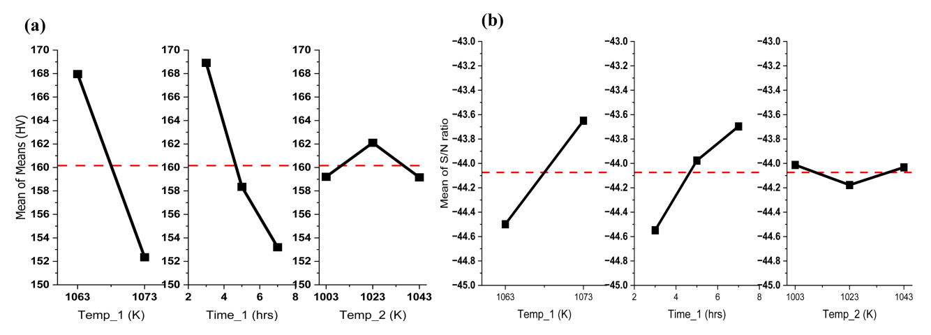
Since ‘the smaller the better’ characteristics of the S/N ratio, the control parameters in the Intercritical annealing such as the 1st heating temperature and time, and the 2nd heating temperature affect the results, they were further analyzed. Table 7 shows the S/N ratio values for each control parameter under the steel Intercritical annealing conditions. Temp_1 refers to the 1st heating temperature, Time_1 refers to the 1st heating time, and Temp_2 refers to the 2nd heating temperature. Each level shown in Table 7 refers to the conditions for each control parameter, as shown in Table 3. The S/N ratio value of each level is expressed as an average of the S/N ratio values of corresponding conditions. For example, the S/N ratio of Level 1 to Temp_1 is the average value of the S/N ratio from IA_1 to IA_9. In Table 7, Delta is the difference between the maximum value and the minimum value of each control parameter. The larger the Delta, the more the parameter affects the surface hardness [25]. This means that the degree to which the control parameter affects the result is more dominant and prioritized, rather than being compared with quantitative figures. According to Table 7, under the steel Intercritical annealing conditions, since the Delta of Temp_1 and Temp_2 is 0.85, the 1st heating temperature and time have a very dominant and preferential effect on the surface hardness compared to other control parameters. Therefore, when considering the spheroidization heat treatment conditions, changing the 1st heating temperature and time rather than the 2nd heating temperature can lead to more changes in the surface hardness.
Fig 9 (a) is a graph of the data in Table 5. In Fig 9, the red dotted line is the average surface hardness value of all 18 conditions. In the case of Temp_1, as the temperature increases, the surface hardness decreases. And in the case of Time_1, as time increases, the surface hardness decreases. However, Temp_2 does not show a tendency according to temperature.
Fig 9 (b) is a normalization of Fig 9 (a) using the S/N ratio. As the slope of each parameter deviates from the dotted red line, which is the average of the S/N ratio, the influence of each parameter increases. The slopes of Temp_1 and Time_1 are generally similar, while the slope of Temp_2 is relatively low and close to the dotted red line. Hence, the S/N ratio analysis of the steel under Intercritical annealing conditions confirmed that the 1st heating temperature and time had the most dominant influence on the surface hardness, and the influence of the 2nd heating temperature was low.
3.4 ANOVA using the surface hardness according to the Intercritical annealing conditions
Using ANOVA, it is possible to confirm whether each control parameter independently affects the result, or how quantitatively each parameter affects the result. The purpose of ANOVA is to determine which control parameters significantly affect surface hardness [25]. The ANOVA is calculated by separating the total variability (Seq SS) of the S/N ratio, the sum of the squared deviations, from the total mean value (Seq MS) of the S/N ratio [23, 26]. For ANOVA, multiple data groups are generated according to each control parameter. If the variance within the data group is very large, the average of samples selected from the data will be different by chance. ANOVA not only analyzes the variance within the data group, but also considers the difference between the sample size and the sample average. All of these factors are expressed as an F-value, and the statistical significance of the F-value is judged through its p-value. In other words, the F-value is used as a test statistic in ANOVA, and the larger the F-value, the larger the average of the data group is compared with the total average. Applied to this research, if there is a control parameter with the largest F-value, the change in the value of the control parameter will have a much greater effect on the average surface hardness (total average).
Table 8 shows the results of ANOVA calculated using the R program. The types of parameters are largely divided into main effects and interaction effects. The interaction effect is an expression of the influence of the parameters on the main effect when they interact with each other. In the main effect, the F-value and the p-value of each parameter may be compared. The p-value decreases as the F-value increases, and the significance of the analysis result can be determined by comparing it with the confidence level, which evaluates whether the F-value is statistically significant.
Temp_1 had an F-value of 30.44, a p-value of 0.005, Time_1 had an F-value of 10.69, and a p-value of 0.025, which is below the confidence level. So, both parameters are statistically significant. However, for Temp_2, the F-value was 0.48 and the p-value was 0.653, which is much larger than the confidence level of 0.05. Hence, Temp_2 is not statistically significant and has no major effect on the surface hardness. In the interaction effect, since the p-value of all interaction parameters is larger than 0.05, none of them were statistically significant, and do not have a major effect on the surface hardness. That is, the parameters of Temp_1, Time_1, and Temp_2 did not show an interaction effect and independently affect the surface hardness.
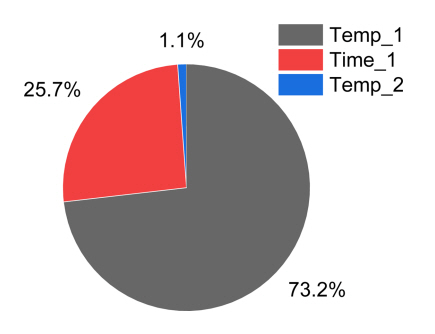
Through the F-value of the ANOVA result, it is possible to quantitatively express the influence of each parameter on the result. According to Table 8, the interaction effect between parameters is significantly lower than that of the main effect, so it can be sufficiently ignored. So, the F-values for the main effects of Temp_1, Time_1, and Temp_2 were calculated as contributions to the results, which are shown in Fig 10. According to Fig 10, Temp_1 shows a distribution of 73.2%, Time_1 shows 25.7%, and Temp_2 shows 1.1%.
In the S/N ratio analysis, the order of effects on Temp_1 and Time_1 was the same. However, the quantitative contribution of the effect through ANOVA differed by about 2.85 times. Therefore, when comparing the two results, Temp_1 has a greater effect on the surface hardness than Time_1, and Temp_1 should be considered first when considering spheroidization heat treatment conditions for decreasing the surface hardness.
In addition, when the three control parameters were divided into the 1st heating process and the 2nd heating process, the effect of the 1st heating process on the surface hardness was very dominant. Applying the spheroidization heat treatment mechanism of Intercritical annealing to this, heating temperature has a more dominant influence than heating time when some cementites in the pearlite are dissolved in the 1st heat treatment step to form austenite. In the 1st heat treatment step, the final surface hardness is greatly affected by how high the heating temperature is set, the energy for dissolution, so that some cementite in the microstructure is dissolved and some cementite remains to act as a nucleus for spherical particles.
4. CONCLUSIONS
Using DSC, it was possible to calculate the trans-formation temperatures of the steel, Ac1 and Ac3 . Ac1 and Ac3 of the steel are affected by the heating rate. In this research, DSC was analyzed at a heating rate of 5 K/min in the spheroidized heat treatment condition. The Ac1 for steel is 1048 K and the Ac3 is 1083 K.
The spheroidization heat treatment conditions of the steel were divided into Subcritical annealing and Intercritical annealing approaches. The resulting surface hardness for each condition was compared. In Subcritical annealing, the condition was best when heat treatment was performed at 1043 K for 20 hours, and the surface hardness value was 140 HV. For Intercritical annealing, the condition was the best when the 1st heating process was performed at 1073 K for 7 hours and the 2nd heating process was performed at 1003 K for 3 hours, and the surface hardness value was 138 HV.
Therefore, considering machinability and process cost, the Intercritical annealing was more suitable for the spheroidization heat treatment of the steel than the Subcritical annealing.
A quantitative analysis method was presented that can compare each condition, by measuring the degree of spheroidization. In the Intercritical annealing, there was a correlation between the spheroidized cementite volume fraction and the surface hardness. The method for measuring the degree of spheroidization includes a spheroidal ratio and a spheroidized volume fraction. An appropriate measurement method is required for each spheroidization mechanism. The spheroidal ratio is a method of measuring the degree of spheroidization suitable for Subcritical annealing, and the spheroidized volume fraction is a method of measuring the degree of spheroidization suitable for Intercritical annealing.
9 of the 18 conditions of the Intercritical annealing were arbitrarily selected and the microstructure of spheroidized particles was photographed using SEM. As a result of a Pearson correlation analysis, the correlation coefficient was determined to be -0.882, which was a very strong negative correlation between the spheroidized cementite volume fraction and the surface hardness.
The degree to which the control parameters in the Intercritical annealing affect the surface hardness was calculated using the S/N ratio and ANOVA. As a result of the S/N ratio, the Delta of the 1st heating temperature and time was 0.85, and the Delta of the 2nd heating temperature was 0.16, which had a preferential effect on surface hardness compared with the 2nd heating temperature.
As a result of the ANOVA, the 1st heating temperature was determined to have the most influence on surface hardness, 73.2%, with the 1st heating time, 25.7% and the 2nd heating temperature, 1.1%. Particularly, when Temp_1 and Time_1 were compared in the 1st heat treatment step, the contribution to Temp_1 was about 2.85 times, compared to Time_1. In the 1st heat treatment step, a change in heating temperature, the energy for dissolution, can result in the optimal transformed microstructure for spheroidization, with only a minimum annealing time for transformation of the microstructure.
Therefore, when it is necessary to lower the surface hardness of the steel using Intercritical annealing, the spheroidization heat treatment condition should be designed by considering the 1st heating temperature and time above the 2nd heating temperature.